I wrote a graphics paper that was published by the Journal of Computer Graphics Techniques. This is the a hopefully simple explanation of it.
You can find the paper here (PDF).
The abstract
While developing Papaya, I looked at how existing image editors implement brushing. I found that most of them compute the Bresenham line joining the last mouse position, and its current position. Then they add the brush stamp along that line.
The GPU repeatedly writes to memory wherever the stamps overlap, which is bad for performance. This is also a classic problem in 3D realtime graphics, and is called overdraw.
The paper attempts to address this problem by rendering a single quad every frame instead of the many overlapping ones in the classic approach.
A simple explanation of the paper
A brush stroke is controlled by four parameters:
- The diameter of each circular brush stamp, in pixels.
- The hardness controls how pixel alpha falls off with distance from the center for each stamp.
- The opacity controls the maximum alpha of the brush stroke. No matter how much you drag the brush around, the value will not exceed the opacity, until you release the mouse and start a new stroke.
- The flow controls how much each stamp adds to the stroke. If you have a low flow, the stroke will get more intense as you repeatedly drag the mouse over the same area. The maximum intensity is clamped to the value of opacity.
Here’s a brush stroke with a low flow. Note how the left and the right pixels are less intense because they are overlapped by fewer stamps. This is also true to a lesser extent for the pixels on the upper and lower edges of the stroke.
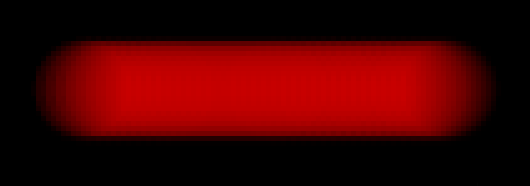
Observe that the intensity at each pixel on the stroke depends on how many stamps overlapped it. The pixels on the far right and left of the stroke are only overlapped by one stamp and hence are the faintest. The pixels along the central stroke axis are stamped by a diameter amount of pixels.
The key insight of the paper is to model a stroke as if the stamp was continuously slid across the central stroke axis, instead of the traditional way of treating stamps as discrete additive blends.
In our new model, the stamp slides horizontally along the middle of the stroke. So the stamp is always at a point , where varies as the stamp slides.
For any given pixel in our stroke, we compute the function , which gives us the instantaneous alpha value contributed to that pixel when the center of the stamp is at .
As the stamp slides from left to right, any given pixel is only inside the circular stamp for a finite amount of time. Stamps in the middle of the stroke stay inside for the longest, and hence have the most intensity.
We can find the centers of the first and the last circular stamp that touched any given pixel. Let’s call the first (left-most) center and let’s call the last (right-most) center . This means that our pixel was inside the stamp as the stamp moved horizontally from to .
Now, we can simply integrate over these two centers, and get the total alpha (i.e. intensity) that a pixel experienced while it was inside the sliding stamp:
The alphabets here can get a bit confusing, so here’s a recap:
- are the coordinates of a pixel. They correspond to the UV coordinates in our pixel shader.
- is the center of the sliding stamp. We integrate over .
- and are constant for any given pixel. They can be computed. They define the interval that we care about, and are the limits of our integral.
- is the function that gives us the instantaneous intensity experienced by point when the stamp is at .
By doing this, we can compute the intensity at a point in one go, without having to repeatedly write to texture memory. This means we’re doing additional computations to reduce memory usage, which is usually a good thing.
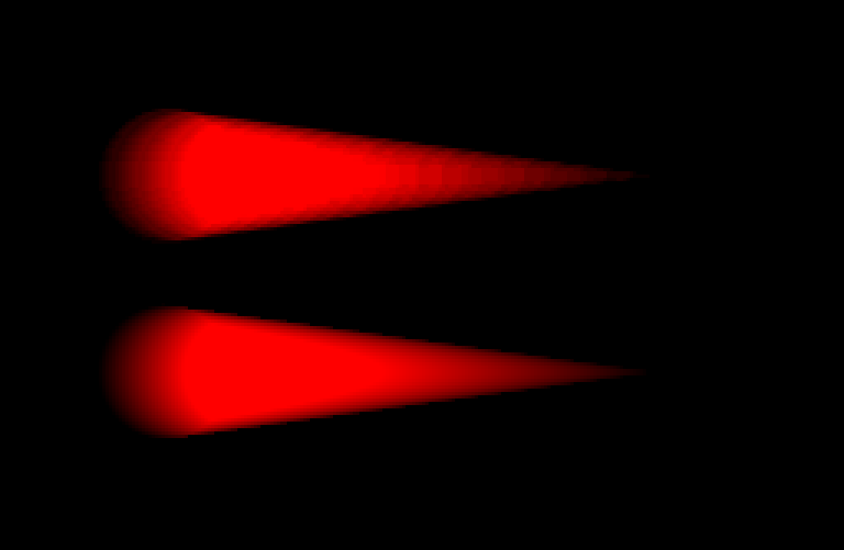
With this technique, multiple strokes line up perfectly when blended additively as seen below. There are two strokes here, but you cannot tell them apart when they become the same color. This means we can get smooth, arbitrarily shaped strokes using chained line segments, which was not possible using my initial distance-based shader.
The paper describes how to compute these things when brush diameter, hardness and flow vary along the stroke, as is required when using pressure-sensitive input devices.
The “Our Approach” section in the paper combines all of these concepts into a succinct list of formulae that directly map to a pixel shader. If you find the math scary, be sure to read the appendices; they are a lot friendlier.
To reiterate, you can find the paper here (PDF).
The paper has pretty comparison images. Be sure to check them out! Here are a few teaser images comparing the discrete method (top) vs this approach (bottom):