In this article, I’m going to try to make it intuitively obvious how digital signal processing and probability theory are deeply connected.

None of what’s presented is even remotely novel math, but I realized it independently about a year ago, and found it to be very beautiful. It connects seemingly disparate disciplines, and it is practically useful in computer graphics.

Convolution

Convolution is a math operation performed on two functions, that produces a third function as an output. The $*$ operator represents convolution, and is defined as:

$f(t) * g(t) = \int f(\tau)g(t - \tau) d\tau$

Arithmetic intuition: When two functions are convolved, you flip one function and then slide it over the other, computing the dot product at every step.

Geometric intuition: You flip one function, slide it over the other and plot the overlapping area at every step.

Here’s two box functions convolved with each other:

Source

Here’s a box function convolved with a decaying impulse:

Source

Convolution is a cornerstone of digital signal processing, Convolution chapter [PDF] from the book The Scientist and Engineer’s Guide to Digital Signal Processing by Steven W. Smith. powering everything from image filters to neural networks.

Probability

Let’s roll a die twice. Let’s call the results of these rolls $X$ and $Y$. These are independent random variables, since one roll does not affect the other.

Let’s plot $P(X)$, which is the probability mass function of the first roll:

$P(X)$ shows that there’s $1/6^{th}$ probability that X is in the range $[1, 6]$, and that there’s zero probability outside this range. Of course, $P(Y)$ will be identical.

Now, let’s look at $P(X + Y)$, which is the probability mass function of the sum of the two rolls:

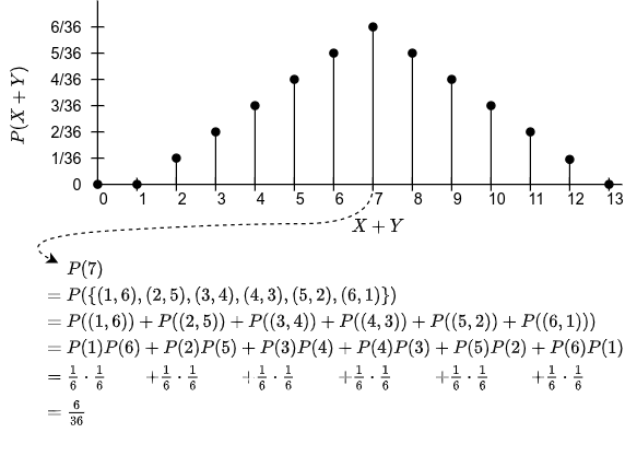
It’s a triangle!

There’s zero probability that $X+Y$ is outside the range $[2,12]$.

There’s a low probability that $X + Y = 2$, because this would only happen if you rolled a 1 followed by another 1. Same goes for 12 (6, 6).

There’s a high probability that $X + Y = 7$, because many pairs of rolls make this possible, as illustrated.

If you actually look at this logic, it is identical to the convolution $P(X) * P(Y)$! We’re flipping one probability mass function and then taking its dot product with the other.

To put this in notation,

$P(X + Y) = P(X) * P(Y) \text{\quad ... (eq. 1)}$

Again, this is a very well understood but beautiful result, tying together basic probability theory on the left hand side, with digital signal processing on the right.

While this is mathematically straightforward, I think it’s useful to have access to both of these isomorphic intuitions.

Side note: Central limit theorem

The central limit theorem is an important result in probability theory. It says that as you sum increasing amounts of random variables from any This is actually a lie. There are some distributions—e.g. famously, the Cauchy distribution—that do not converge to Gaussians. distribution, the resulting probability distribution tends towards a Gaussian distribution.

In other words, the following functions tend towards Gaussians:

$\begin{aligned} &P(X + Y + Z + ...) &&\textit{according to the central limit theorem} \cr =\space &P(X) * P(Y) * P(Z) * ... &&\textit{according to (eq. 1)} \cr =\space &P(X) * P(X) * P(X) * ... &&\textit{since X, Y, Z come from the same arbitrary distribution} \cr \end{aligned}$

This means that repeatedly convolving a function with itself will converge towards a Gaussian.

While I’m currently incapable of bringing concrete “aha!” moments to the table about the central limit theorem, it’s a result that is deeply related to the isomorphism in equation 1, and is fun to think about.

Applications

This concept is useful for shaping the probability mass function of randomness/noise. E.g. if you sample uniform noise twice, and sum the two samples, you get triangular noise, which is used to reduce quantization-banding in images. Banding in Games: A Noisy Rant [PDF] (slides 27-30) by Mikkel Gjoel.

Another cool paper Filtering by repeated integration by Paul S. Heckbert. talks about using summed area tables to enable variable-width FIR (finite impulse response) filtering. Even these words mean nothing to you, the key takeaway is that the paper uses this isomorphism. It even briefly touches on how these concepts are related to splines!

That’s all I have for now. Hope this intuition is helpful to you.